Making Thematic Maps and Census Data Work for IR

Illustrating Geographical Distributions and Describing Populations Using Data from the U.S. Census Bureau

In a previous post I give an example and step-by-step instructions for the geocoding process (converting street address locations to lat/long coordinates). In another previous post I give an example and step-by-step instructions on how to use QGIS to illustrate the spatial distribution of geocoded addresses as a point and choropleth map as well as how to perform a ‘spatial join’ that will identify each location with an associated geography (using a geo identifier for Census tract, zip code, legislative district, etc – whatever your geographic level of interest).

In the current post, using ArcMap rather than QGIS (though it is the same conceptual process), I provide an example and step-by-step instructions for taking this one step farther and joining actual U.S. geography-based Census demographic data to the address locations file without ever leaving the ArcMap platform.

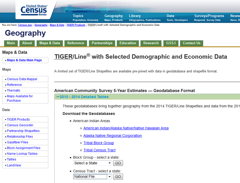
Step 1, Download the Tract Shape and Data File: The U.S. Census Bureau provides downloads that contain both the tract level shape file (the underlying map) along with selected demographic and economic data. These data are derived from the American Community Survey (ACS) and are presented as five-year average estimates since the ACS is carried out through sampling and it requires a five year pooling of the data to arrive at reasonably accurate estimates. In this case I have elected to download the national file that reflects the most recent 2010-14 tract level data estimates. Click here for a direct link to the U.S. Census Geodatabases page.

tiger-file-download

Continue reading Making Thematic Maps and Census Data Work for IR

Visualizing Survey Results: Class Discussion by Class Year

Jason Bryer, a fellow IR-er at Excelsior College has a nice post (link) about techniques for visualizing Likert-type items – those “Strongly disagree…Strongly agree” items only found on surveys.  He has even been developing an R software package called irutils that bundles these visualization functions together with some other tools sure to be handy for anyone working with higher ed data.

Jason’s post reminded me that I have been meaning to try out a “fluctuation plot” to visualize some recent survey results.  A fluctuation plot, despite the flashy name, simply creates a representation of tabular data where rectangles are drawn proportional to the sizes of the cells of the table.  The plot below has responses to a question about how often students here participate in class discussion along the left side and class year along the bottom.  The idea behind this is to have a quick and very intuitive way to visualize how this item differs (or doesn’t differ) by class year.  In this case, it looks like fewer of our sophomores (as a percentage) report participating in class discussion “very often” than their counterparts.  This may suggest a need for further research.  For example, are there differences in the kinds of courses (seminar vs. lecture) taken by sophomores?

Creating the plot

The plot itself requires only one line of code in R.  If you are not a syntax person, I recommend massaging the data as much as possible in a spreadsheet first.  You can take advantage of a default setting in R where text strings are converted to “factors” automatically.  This default functionality usually annoys the daylights out of R programmers, but in this case, it is actually exactly what you want.

All you need to do is set up your data like this:

Then you can save the file as a .csv and import it into R using my preferred method – the lazy method:

mydata<-read.csv(file.choose())

Nesting file.choose() inside of the read.csv() function brings up a GUI file chooser and you can just select your .csv file that way without having to fiddle with pathnames.

Once you’ve done this, you just need to load (or install then load) the ggplot2 package and you can plot away like this:

ggfluctuation(table(mydata$Response, mydata$Year))

You can add a title, axis labels, and get rid of the ugly default legend by adding some options:

ggfluctuation(table(mydata$Response, mydata$Year)) + opts(title=”Participated in class discussion”,  legend.position=”none”) + xlab(“Class year”) + ylab(“”)

Once you’ve done that, you’ll have just enough time left to prepare yourself for the holiday cycle of overeating-napping in front of the TV-overeating some more.  My family will be having our traditional feast of turkey AND lasagna.  If your life so far has been deprived of this combination, I suggest seeking out someone of Southern Italian heritage and inviting yourself over for dinner.  But be warned – you may be required to listen to Mario Lanza records during the meal.

Happy Thanksgiving!

The WSJ’s “From College Major to Career”

WSJ Major to Career

I am a regular reader of Gabriel Rossman’s blog, Code and Culture.  He posted an analysis yesterday (Nov. 7, 2011) featuring data from an interactive table published in The Wall Street Journal in a series entitled “Generation Jobless.”  The interactive data table can be found as a sidebar to the main article called “From College Major to Career.”

Majored in what when?

Given the focus of the “Generation Jobless” series, I just assumed that this interactive table would depict recent grads.  I was curious about the data used to create the table, so I decided to look into it a bit.  As you can see from the description above the table, it is based on the 2010 Census.   But then at the bottom of the table, the Georgetown Center on Education and the Workforce is cited as the source.  I looked around at the Center’s website and I found what I think might be the WSJ’s source and it is a 2011 report called What It’s Worth: The Economic Value of College Majors by Anthony P. Carnevale, Jeff Struhl, and Michelle Melton.  By scrolling to the bottom of the project page, I was able to find a methodological appendix that explains the data that they used in their analysis.  They used the 2009 American Community Survey (ACS) which apparently for the first time ever “asked individuals who indicated that their degree was a bachelor’s degree or higher to supply their undergraduate major” (Page 1).  If you read on in the appendix you see that “the majority of the analyses are based on persons aged 18-64 year old” and that “for the majority of the report we focus solely on persons who have not completed a graduate degree”.  I looked back at the full report and I don’t see a table that has age categories or a subsection devoted to something like “recent grads”.  It also turns out that this report received some press from both The Chronicle and InsideHigherEd when it was published back in May.  Both of these pieces, which cite the director of the Center and one of the authors of the report, Anthony P. Carnevale, say that the data are from 25-64 year olds.  So if the WSJ is using recent grads or an age category other than 25-64, I’m not sure if they’re getting it from this report (at least not directly).  If the WSJ is using 25-64 year olds, you might be like me and this table might not mean what you think it means.  That is, it might not capture how recent grads are faring in the job market these days.  If it reflects all workers with bachelor’s degrees aged 25-64, you could be getting folks at all stages of their careers.  For example, could these data include a 64 year old who majored in Finance, say, 40 years ago?  Is their experience going to be the same as what is facing a member of “Generation Jobless”?

Again, I don’t know for sure how the WSJ used these data.  Maybe someone else out there has had better luck finding out exactly how the folks at the WSJ have created this table?

Degrees by Academic Division 1985-2011

There always seems to be plenty of discussion in higher ed about the shifts in student interest in the academic disciplines and divisions over the years.  The issue has probably taken on a heightened sense of urgency in the last few years with the economic situation, prompting statements about the “death” or “rebirth” of certain disciplines.  So what’s my take on it?  I’d be happy to share some lengthy tome, some 1,000 word screed on the subject, but instead…  Check out the p r e t t y  c o l o r s!

The chart above depicts the percentage of degrees awarded at Swarthmore by academic division.  Percentages are based on the number of majors, so graduates with double majors may appear in more than one division if their majors were in different divisions.  (For more info on degrees, head over to the “degrees” section of our Fact Book page).

In addition to having pretty colors, this chart also happens to be very easy to make in R.  In fact, if your data are arranged properly, which you can always do ahead of time in Excel, this chart can be created using one line of code with the ggplot2 package:

qplot(Year, Percent, data=mydata, colour=Division, geom=”line”, main=”Degrees by Academic Division 1985-2011″)

If you are new to R and you are like me and hate worrying about getting the file path right when reading data into R, save your data as a .csv file and use file.choose:

mydata<-read.csv(file.choose())

You could also just highlight the data in Excel, copy it to the clipboard, and then read it into R, being sure to tell R that the data are tab-delimited:

mydata<-read.table(file=”clipboard”, sep=”\t”)

So there you have it, an increase in pretty colors with a minimum of effort which surely means more time for Angry Birds important stuff.

Speedy PSPP

GNU PSPP logoYes, someone is using that acronym for their software.  And yes, I promise not to make any bad jokes that reference the early 90s rap song, also with an acronym.  If you’re not sure which song I am referring to, so much the better for you.

PSPP is intended as a “free replacement” for SPSS.  Since I’m not a big user of SPSS, I had not paid PSPP much attention until just recently.  The reason I looked at PSPP a second time is that I wanted to quickly open a .sav file (the SPSS native file format) to look at value labels.  We have access to SPSS here at the college, but why PSPP offered an alternative in this situation is that we access a networked version of SPSS which can take some time to open.  PSPP, on the other hand, is very light and can reside on my machine.  So I decided to give it a try and found that I can open data sets very quickly.

I was so impressed with the speed improvement that I changed the .sav file type association on my machine to PSPP.  Of course, what better way to show one’s appreciation!  Now, keep in mind that I do not use SPSS much at all and PSPP only offers what they call a “large subset” of the capabilities of SPSS, so this may not be a suitable replacement for the SPSS overachievers out there.  You can also open .sav files in R using the read.spss command in the foreign package, but if you’re like me and you might want to look at them first, PSPP allows you to do this.  It also offers the opportunity to work with SPSS files at home, for those of us for aren’t going to want to purchase an SPSS license for the home computer.

If others have PSPP experiences to share, I’d love to hear them!


Mapping Student Counties

Photo by Aram Bartholl

We thought it might be interesting to create a map of the home counties of our domestic students.  Since this is something that I have seen done in R and I am always up for trying to sharpen my R programming skills, I thought I would give it a shot.

My first step was to retrieve zip codes for all current students from Banner.  I am able to do this using the RODBC package in R.  This requires downloading Oracle client software and then setting up an ODBC connection to Oracle first.  Once this is set up, I can connect to banner, enter my username and password, and then pass a SQL statement to Banner.  Here is the code for this step:


library(RODBC)

prod<-odbcConnect("proddb")

zip<-sqlQuery(prod,
paste("select ZIP1 from AS_STUDENT_ENROLLMENT_SUMMARY where TERM_CODE_KEY=201102 and STST_CODE='AS' and LEVL_CODE='UG'"))

odbcClose(prod)


This creates an R dataframe called “zip” and closes my RODBC connection to Banner. The example that I am following uses FIPS county codes, so I will need to prep these zip codes for use with a FIPS lookup table by first making sure they are only 5 digits. Then I import my FIPS lookup table (making sure to preserve leading zeros) and merge with student zip codes. Once I have done this, I can get the counts of students in each of the FIPS codes.

zip$ZIP<-substr(zip$ZIP1,1,5)

fips<-read.csv("C:/R/FIPSlookup.csv",
colClasses=c("character","character"))

m<-merge(zip, fips, by="ZIP")

fipstable<-as.data.frame(table(m$fips))

Now I can proceed with the example that I am using.  This example comes from Barry Rowlingson by way of David Smith’s “Choropleth Map Challenge” on his excellent, all-things-R blog.  I chose this method because it does not rely on merging counties by name, but instead uses FIPS codes – which we now have thanks to the steps above.

Then I use the “rgdal” package to read in US Census shapefile (available here), prep the FIPS codes in the shapefile and match with our student counts, and assign zeros to counties with no students:

library(rgdal)

county<-readOGR("C:/Maps","co99_d00")
county$fips<-paste(county$STATE,county$COUNTY,sep="")

m2<-match(county$fips,fipstable$Var1)
county$Freq<-fipstable$Freq[m2]
county$Freq[is.na(county$Freq)]=0

Following Rowlingson, we use the “RColorBrewer” package and his own “colorschemes” package to get the colors for our map and associate them with counts of students. We then set the plot region with blank axes, add the counties, and then draw the plot:

require(RColorBrewer)
require(colourschemes)

col<-brewer.pal(6,"Reds")
sd<-data.frame(col,values=c(0,2,4,6,8,10))
sc<-nearestScheme(sd)

plot(c(-129,-61),c(21,53),type="n",axes=F,xlab="",ylab="")
plot(county,col=sc(county$Freq),add=TRUE,border="grey",lwd=0.2)

Click the thumbnail below to see the resulting map:

As you can see, the map is pretty sparse as you might expect with 1531 students from 325 different counties.  This represents only a first pass at trying this, so there will be more to come, possibly a googleVis version.  If others have had success with the above approach, we would love to hear about it in the comments!

To get more info about the geographic distribution of our students (both international and domestic), check out the “enrollments” section of our Fact Book page here.

The R syntax highlighting used in this post was creating using Pretty R, a tool made available by Revolution Analytics.