Illustrating Geographical Distributions and Describing Populations Using Data from the U.S. Census Bureau
In a previous post I give an example and step-by-step instructions for the geocoding process (converting street address locations to lat/long coordinates). In another previous post I give an example and step-by-step instructions on how to use QGIS to illustrate the spatial distribution of geocoded addresses as a point and choropleth map as well as how to perform a ‘spatial join’ that will identify each location with an associated geography (using a geo identifier for Census tract, zip code, legislative district, etc – whatever your geographic level of interest).
In the current post, using ArcMap rather than QGIS (though it is the same conceptual process), I provide an example and step-by-step instructions for taking this one step farther and joining actual U.S. geography-based Census demographic data to the address locations file without ever leaving the ArcMap platform.
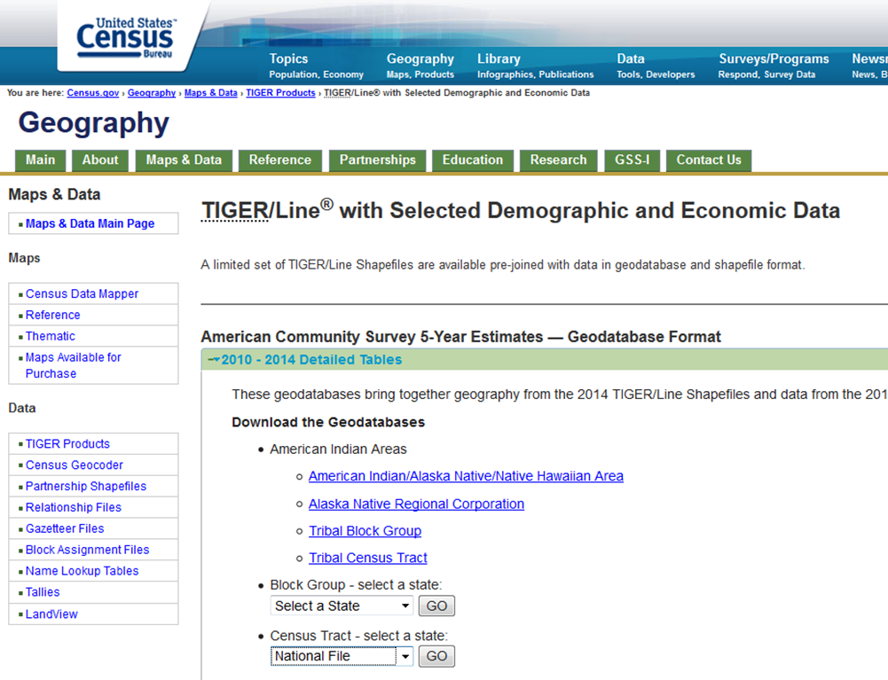
Step 1, Download the Tract Shape and Data File: The U.S. Census Bureau provides downloads that contain both the tract level shape file (the underlying map) along with selected demographic and economic data. These data are derived from the American Community Survey (ACS) and are presented as five-year average estimates since the ACS is carried out through sampling and it requires a five year pooling of the data to arrive at reasonably accurate estimates. In this case I have elected to download the national file that reflects the most recent 2010-14 tract level data estimates. Click here for a direct link to the U.S. Census Geodatabases page.
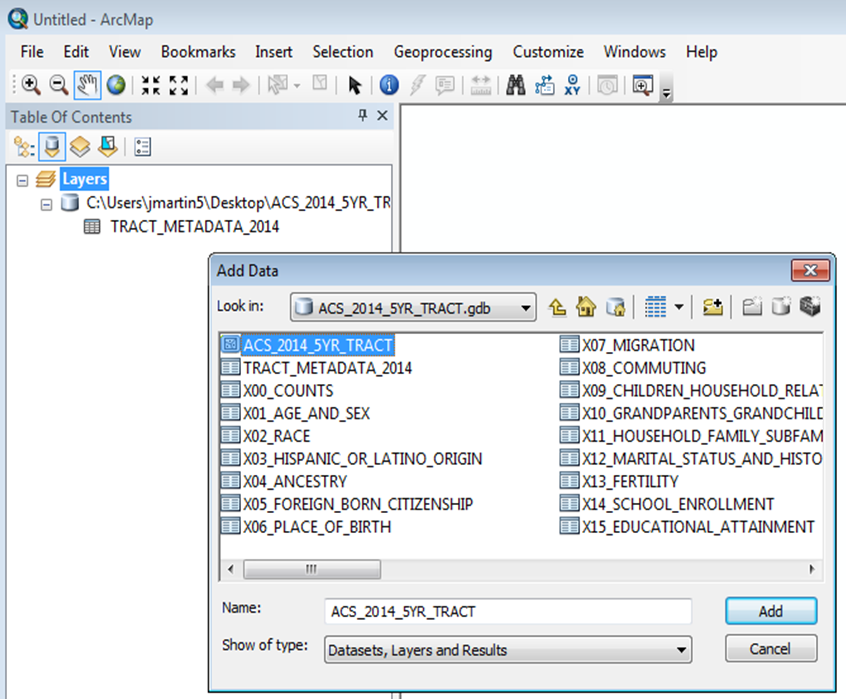
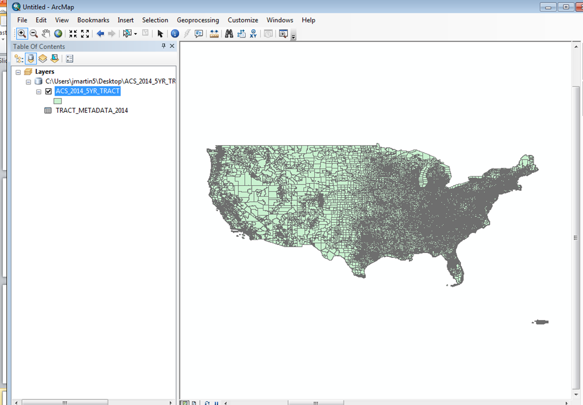
Step 2, Upload the Tract Shape File to ArcMap: The U.S. Census download contains multiple files, including the tract shape itself, much of the available tract level data, and a meta data file that labels/describes the available variables. By uploading/adding “ACS_2014_5YR_TRACT” you will be uploading the empty shape or polygons that represents the more than 74,000 tracts in the U.S.
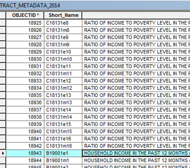
Step 3, Upload the Census Meta Data File: To determine which variables you are interested in, you will need to upload/add and open the “TRACT_METADATA_2014” file from the Census download. In this case, I have highlighted the Median household income estimate among the thousands of available variables and variable combinations.
Step 4: Upload Geocoded Address File: Now that our shape file and meta data are uploaded/added, we need to do the same to our geocoded address file. These lat and long coordinates can be added to the ArcMap document in the same way we added the shape file and meta data. ArcMap will recognize a variety of file types for this (Excel, text, CSV, dbf, etc.)
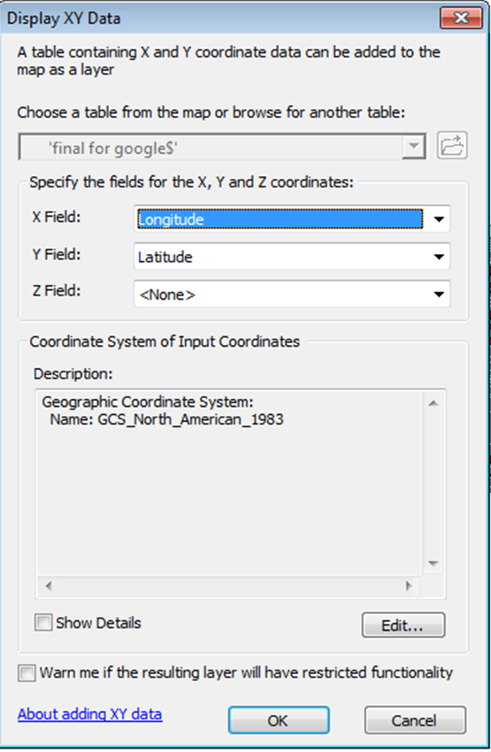
Step 5: Displaying X/Y Data: With the address data uploaded, we can plot the points on the map itself by right-clicking on the data in the left-hand margin and choosing “Display XY Data.” This will create an “events” layer with the point locations and will plot the data points on the map of Census tracts.
 Step 6: Export “Events” as a “Shape File”: In order to prepare our “Events” layer to be spatially joined to the underlying tracts, we have to export it as a shape. By right-clicking -> data -> export data, we will both save and add an export layer to the ArcMap Document that can then be joined to the tract file (since the events layer cannot itself be joined).

Step 7: Spatial Join – (Locations to Tract File): Ultimately, we are going to join the address locations to the tract file (showing how many addresses fall in each tract) and join the tract file information to the address locations (showing the tract “Geo ID” associated with each address), but I will start by describing the former (addresses to tracts).
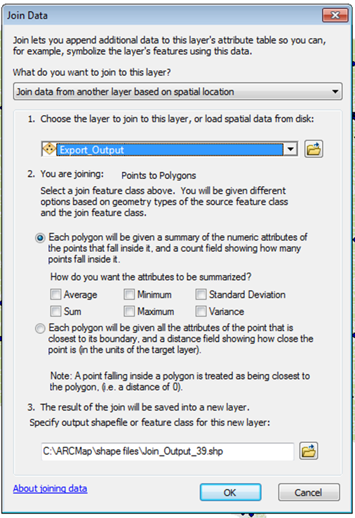
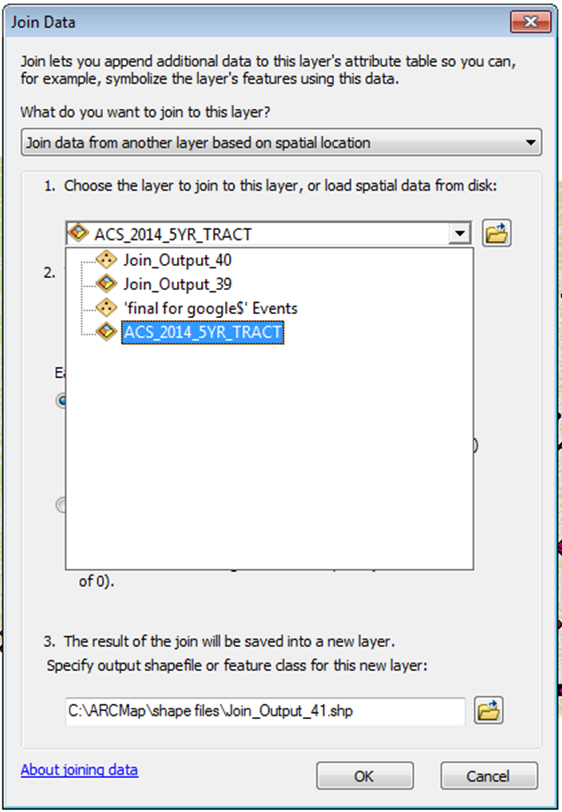
If we right-click on the tract layer file “ACS_2014_5YR_TRACT,” it will give us the option of selecting a “join.” We want to “Join data from another layer based on spatial location.” The layer we want to join to our tract layer is our newly created “Export_Output” which is our point locations layer. We also want to select the option for each polygon to be given the numeric attributes of points that fall inside it and (more importantly) a count field showing how many points fall inside it. In this case, we are not looking for any numerical summation other than the number of addresses inside each tract. 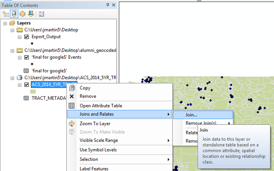
 The result is a “Join Output” layer that now includes, in its attributes table, a count of the number of addresses found in each Census tract.
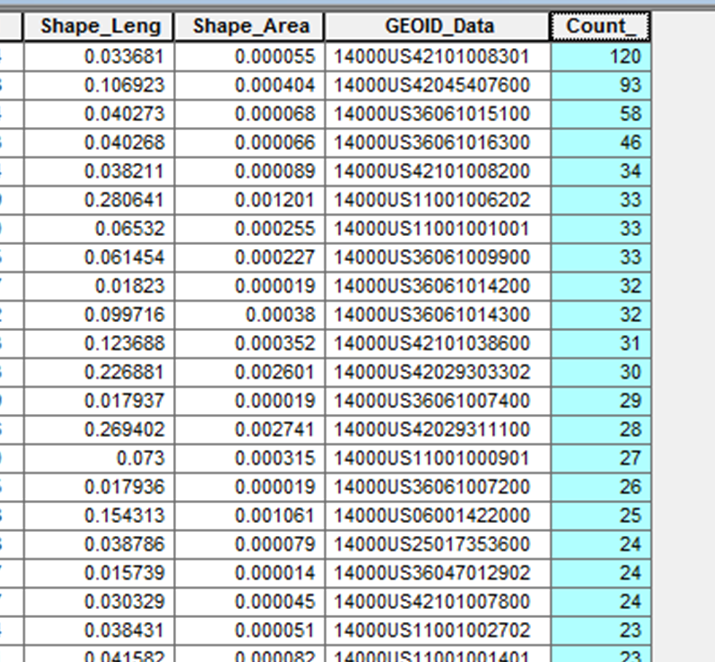
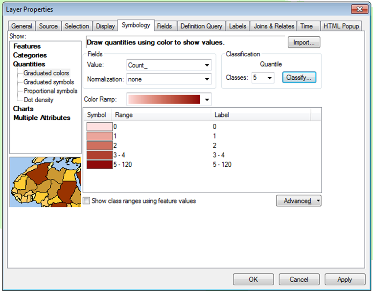
Step 8, Creating a Choropleth Map: If we now want to create a choropleth (color shaded) map that reflects the concentration of addresses across the country, we right-click on the new “Join Output” file and select “Properties.” Under the “Symbology” tab, we can select “Graduated colors,” and under “Fields -> Value” we can scroll down to our variable of interest, “Count.” We can also adjust break points, color preference, etc. from this window.
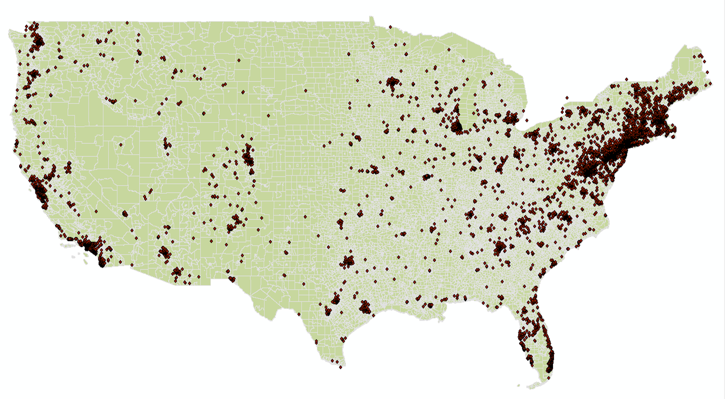
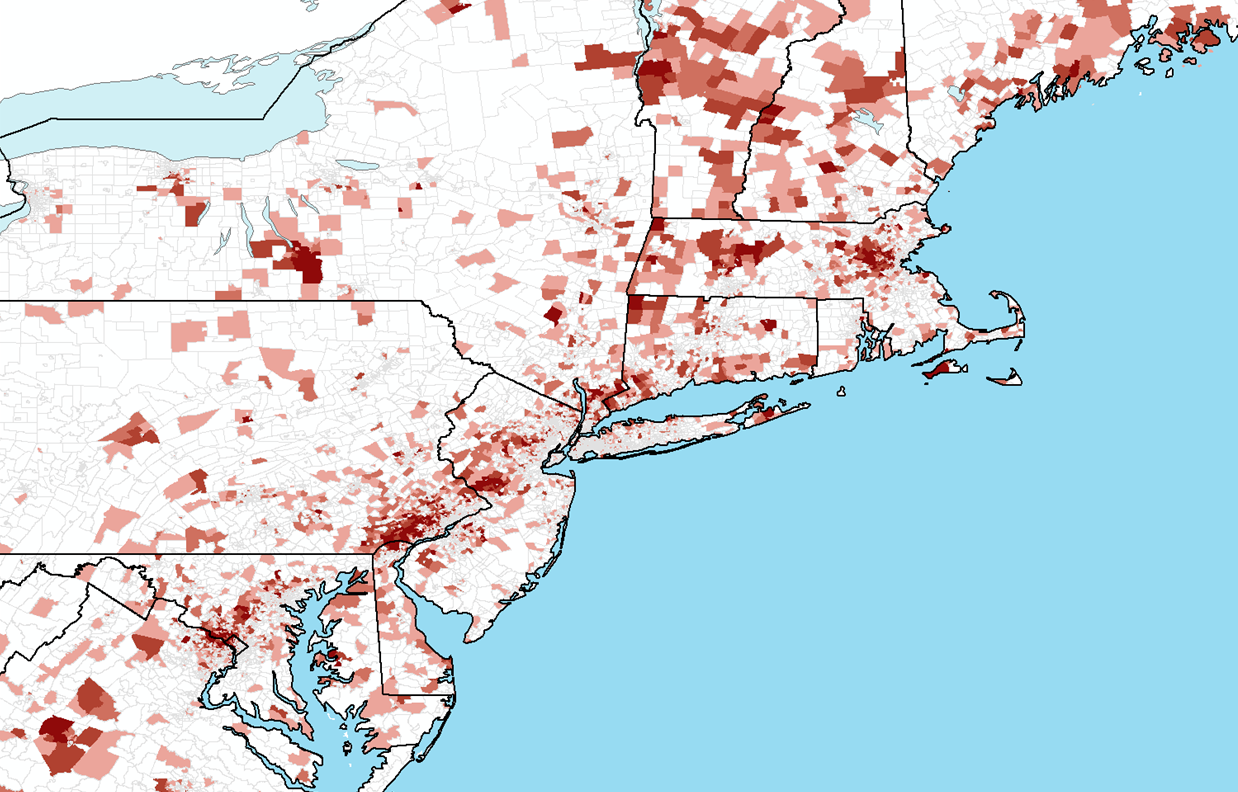
Step 9, Zooming to Desired Level, Adding State Lines, Oceans, etc: After the choropleth map is created, we can can explore adding additional boundaries, shapes etc, as well as adding and formatting an appropriate legend if you wish. This image can be exported in variety of formats, including jpeg and Adobe Illustrator format.
Step 10: Spatial Join (Tract File to Locations): In step seven I mentioned that we will also be joining the tract file information to the address locations (showing the tract “Geo ID” associated with each address). The ultimate purpose is to incorporate Census neighborhood description characteristics (such as the median income) into each of the individual entries on our address file.
In this case, we start with our “Export_Output” file (which is the layer that contains are plotted address points). We carry out another spatial join where we select the tract shape file “ACS_2014_5YR_TRACT” to join to the plotted address points. In this case, we want the result of the join to include all of the shape file characteristics as new columns/variables in our “Export_Output” file. The central thing we accomplish by doing so is adding the identifier (Geo ID) of the tract that contains each one of the addresses to the original address file.
Step 11, Uploading the Appropriate Census Data File to ArcMap: Now that we have the tract “Geo ID” associated with each address listed in a new “Join Output” layer, we can go one step farther and connect specific Census data to that file based on the common “Geo ID” variable. To upload, we again “Add Data” and return to our original Census download (the geodatabase files from the beginning). This download divides the thousand of variables and variable combinations into topic areas. I know that the variable I am interested in from back when I reviewed the meta data can be found in the income subset so that is the one I loaded into ArcMap.

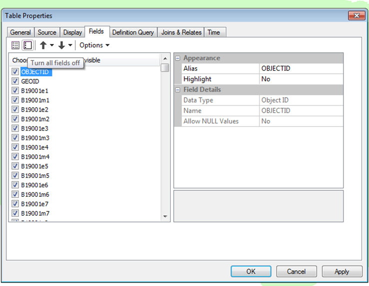
Step 12, Trimming Income Data to Desired Variables: Because these files contain so many variables, the system can get bogged down if we do not focus in on those we want to keep. In this case, after uploading, I have right-clicked on the “X19_Income” data and gone to “Properties.” From here I can select the “Fields” tab, turn off all fields, and then add back the ones that I need (in this case my median income variable and the “GeoID” variable so I can join it to my addresses).
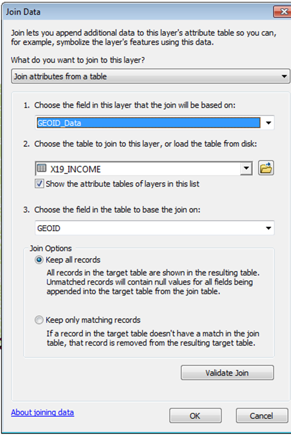
Step 13, Joining Income Data to Address File Based on GEO ID: Now that we have all the necessary data components, we could export everything and merge the data in our stats software of choice, but we can also do it right here in ArcMap. This is another join – just not a spatial join this time. If we return to our “Join_Output” file (the one where we joined the GeoID to our address file), we right-click again and “join” again. This time we will choose to “Join attributes from a table” instead of doing a “spatial” join. We then select the “X19_Income” table to join, and select the GeoID variables from each table as the field to join on.
 Step 14: Exporting Data to a Spreadsheet: The resulting join is a table with all of our original addresses, the associated tract identifier, and the median income for that Census tract as reported in the 2010-14 five year estimates. We can export this spreadsheet by opening the attribute table for the join, navigating to the icon in the upper left hand corner, clicking and selecting “Export” on the menu that opens. When saving, it is important to remember to save as “dbase Table” rather than the default setting, “File and Personal Geodatabase tables.” If you do the latter it will result in an error. If you do the former it will download a DBF table that can be uploaded into Excel or elsewhere.
These data can then be merged with any additional data you have on the individuals represented by the addresses as well as any additional neighborhood information you have on those tracts.
An important thing to remember when interpreting and analyzing this data is that the Census data describe the neighborhoods of the individuals who live there and not the individuals themselves. If we fail to make this distinction, we commit an ecological fallacy.