National Student Clearinghouse: Degree Title Categories

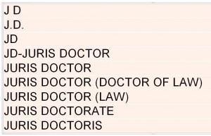
I enjoy working with National Student Clearinghouse (NSC) return data, but the differences between the way schools report Degree Titles can be frustrating.  For example, here’s just a few of the ways “juris doctor” can appear:

a few ways JD can appear

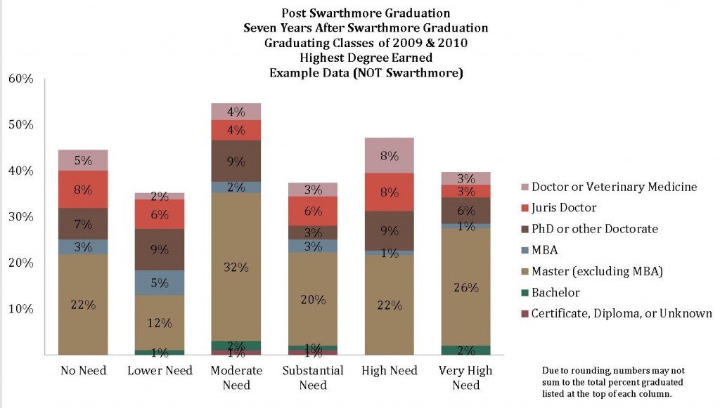
I’ve worked on a few projects where it was necessary to work with the type of degree that was earned.  For example, as part of Access & Affordability discussions, it was important to examine the additional degrees that Swarthmore graduates earned after their Swarthmore graduation by student need level to determine if graduates in any particular need categories were earning certain degrees at higher/lower rates than other need categories.

example data_degree cat by need cat


In order to do this, I first had to recode degree titles into degree categories.

The NSC does make available some crosswalks, which can be found at https://nscresearchcenter.org/workingwithourdata/

The Credential_Level_Lookup_table can be useful for some projects.  However, my particular project required more detail than provided in the table (for example, Juris Doctors are listed as “Doctoral-Professional” and I needed to be able to separate out this degree), so I created my own syntax.

I’m sharing this syntax (below) as a starting point for your own projects. This is not a comprehensive list of every single degree title that has been submitted to the NSC, so be careful to always check to see what you need to add to the syntax.

While I have found this to be rarer, there are the occasional degrees that come through without a title in any of the records for that degree.  I’ve therefore also included a bit of syntax at the top that codes those with a Graduated=”Y” but a blank Degree Title to “unknown.”  If you are choosing to work with those records differently, you can comment out that syntax.

Once you have created your new degree categories variable(s), you can select one record per person and run against your institutional data.  One option is to keep, for those who have graduated, the highest degree earned.  You can use “Identify Duplicate Cases” to Define Matching Cases by ID and then Sort Within Matching Groups by  DegreeTitleCatShort (or any other degree title category variable you’ve created).  Be sure to select Ascending or Descending based on your project and whether you want the First or Last record in each group to be Primary.

Hope this helps you in your NSC projects!

SPSS syntax:  Degree Title Syntax to share v3

Making Thematic Maps and Census Data Work for IR

Illustrating Geographical Distributions and Describing Populations Using Data from the U.S. Census Bureau

In a previous post I give an example and step-by-step instructions for the geocoding process (converting street address locations to lat/long coordinates). In another previous post I give an example and step-by-step instructions on how to use QGIS to illustrate the spatial distribution of geocoded addresses as a point and choropleth map as well as how to perform a ‘spatial join’ that will identify each location with an associated geography (using a geo identifier for Census tract, zip code, legislative district, etc – whatever your geographic level of interest).

In the current post, using ArcMap rather than QGIS (though it is the same conceptual process), I provide an example and step-by-step instructions for taking this one step farther and joining actual U.S. geography-based Census demographic data to the address locations file without ever leaving the ArcMap platform.

Step 1, Download the Tract Shape and Data File: The U.S. Census Bureau provides downloads that contain both the tract level shape file (the underlying map) along with selected demographic and economic data. These data are derived from the American Community Survey (ACS) and are presented as five-year average estimates since the ACS is carried out through sampling and it requires a five year pooling of the data to arrive at reasonably accurate estimates. In this case I have elected to download the national file that reflects the most recent 2010-14 tract level data estimates. Click here for a direct link to the U.S. Census Geodatabases page.

tiger-file-download

Continue reading Making Thematic Maps and Census Data Work for IR

The Importance of IR

Anyone who is not yet convinced about Picture of first page of the Supreme Court decision document.the importance of a strong institutional research office in supporting planning, assessment, and decision-making at colleges and universities today needs only to read Justice Anthony M. Kennedy’s 2016 opinion in the Fisher case on race-conscious admissions to understand:

“The University now has at its disposal valuable data about the manner in which different approaches to admissions may foster diversity or instead dilute it. The University must continue to use this data to scrutinize the fairness of its admissions program; to assess whether changing demographics have undermined the need for a race-conscious policy; and to identify the effects, both positive and negative, of the affirmative-action measures it deems necessary.”

Our profession has evolved over the past 50 years, from a handful of data wonks focused primarily on responding to external agencies’ fledgling efforts to understand the increasingly complex higher education landscape, to internally focused analytic teams, indispensable to institutional decision-making.

An effective IR office uses its data infrastructure to provide basic institutional information to internal and external audiences, and then builds on that essential foundation, leveraging its expertise and perspective to provide meaningful research and analytics that illuminates what is and isn’t working, the results of new initiatives to support students, general educational outcomes, and future directions that may be promising.  To fully support its institution the IR office must go beyond providing reports on topics that faculty and managers are interested in hearing about, and educate about what they ought to know – whether or not it is what they want to hear.  This is essential for evidence-based decision-making, differentiating effective institution from the rest.


Where in the World is Everyone? Part Two

Part Two: From Geographic Location to Neighborhood Profile

In Part One of this two part blog post I explained how to start with a list of street addresses and, using Google’s Fusion Tables function, map those locations onto an interactive Google Map. This tool alone can be very useful and powerful in the context of institutional research and administration. However, where spatial analysis becomes significantly more powerful is when you use these known locations to find out more information about the specific communities and neighborhoods of students and alumni. Through the use of spatial analysis software, these “point” locations can be tied directly to zip codes, census tracts, block groups, Congressional districts, etc. From there, geographic data from the Census Bureau’s American Community Survey or other sources can be used to understand a great deal about where the community and neighborhood profile of students and alumni. It’s only a proxy for the individual and we always need to be aware of the Ecological fallacy, but you can gain immense and detailed understanding of a group just by learning about their spatial location.

geo_2_image_7

The following is a guide for taking individual records (including street addresses), overlaying geographic boundaries (such as tracts, zip codes, etc.), joining (or combining) the individual records with their respective geographic descriptors (e.g. Student A lives in zip code 12345), and finally, joining/combining geography-based data from the US Census’ American Community Survey to those individual records (e.g. Student A lives in zip code 12345, which has a population of 3,500, a median household income of 65,000 dollars per year, and so on).

Continue reading Where in the World is Everyone? Part Two

Where in the World is Everyone? Part One

Part One: Making Use of Mapping in Institutional Research

A good visual can be a helpful tool considering that the job of an Institutional Researcher is to keep the attention of people who have many important things to do with their time and little time to spend wading through a lot of text and long explanations. Enter mapping and spatial analysis. Maps generally make for familiar, easy to read, and aesthetically pleasing images that grab viewers’ attention and, when carefully constructed, do a very good job of communicating information. They are nice to look at, but they can also tell us relevant and important about our institution. I elaborate on a specific technique in this post (Part One) and delve more deeply into the topic in a follow-up post (Part Two). In this post I illustrate a simple but effective technique for mapping point locations. In the following post (Part Two), I discuss some of the potential deeper applications for mapping and spatial analysis in Institutional Research.

Current_Student_Home_Addresses_Continental_US_2014-15

Continue reading Where in the World is Everyone? Part One

The Sport of IR

football game
theunforgettablebuzz.com

I was watching the NFL season-opening  game last night.   I’m not actually a football fan, but when your husband writes a book connected to football, it’s one of the sacrifices you make.  (I have also watched DOTA tournaments with my son, and thought it made about as much sense as professional football.   What can I say, I love my guys.)   I was struck by the between-play graphics of the players and their stats, and got to wondering (it wasn’t as if the game held my attention), what kinds of pictures and stats would be shown on a highlights reel of Institutional Researchers.  (You don’t know, it could happen.) Continue reading The Sport of IR

Video and SPSS Syntax: Deleting Select Cases Using the National Student Clearinghouse Individual Detail Return File

There may be some situations where you would want to delete select records from an individual return file. For example, you may have a project where you are looking at student enrollment after graduation or transfer, and it is decided that your particular project will only include records for which a student was enrolled for more than 30 days in a fall/spring term or more than 10 days in a summer term. Or, you may have six years of records for a particular cohort, but you only want to examine records for four years. In both of these cases, you would want to delete the records that don’t fit your criteria before analyzing your data.

Continue reading Video and SPSS Syntax: Deleting Select Cases Using the National Student Clearinghouse Individual Detail Return File

Video and SPSS Syntax: Admit/Not Enroll Project Using the National Student Clearinghouse Individual Detail Return File

Irish United Nations Veterans Association house and memorial garden (Arbour Hill)” by Infomatique is licensed under CC BY-SA 2.0

I use the National Student Clearinghouse individual detail return file and SPSS syntax in this video to capture the first school attended for students who were admitted to my institution, but who did not enroll (names listed are not real applicants). In a future video, I’ll work on the same project using the aggregate report. I almost always use the individual detail return file since it provides so much information, but it does have a limitation that impacts this project.

Continue reading Video and SPSS Syntax: Admit/Not Enroll Project Using the National Student Clearinghouse Individual Detail Return File

Decisions, Decisions

I’ve been working with data from the National Student Clearinghouse (NSC) for a while now. A lot of wonderful information can be found in the NSC data, but the detailed return file can sometimes be a bit difficult. There are so many ways the data can be sliced, and it can sometimes be challenging to determine how best to work with the data to present meaningful information to stakeholders.

Continue reading Decisions, Decisions