Part Two: From Geographic Location to Neighborhood Profile
In Part One of this two part blog post I explained how to start with a list of street addresses and, using Google’s Fusion Tables function, map those locations onto an interactive Google Map. This tool alone can be very useful and powerful in the context of institutional research and administration. However, where spatial analysis becomes significantly more powerful is when you use these known locations to find out more information about the specific communities and neighborhoods of students and alumni. Through the use of spatial analysis software, these “point” locations can be tied directly to zip codes, census tracts, block groups, Congressional districts, etc. From there, geographic data from the Census Bureau’s American Community Survey or other sources can be used to understand a great deal about where the community and neighborhood profile of students and alumni. It’s only a proxy for the individual and we always need to be aware of the Ecological fallacy, but you can gain immense and detailed understanding of a group just by learning about their spatial location.
The following is a guide for taking individual records (including street addresses), overlaying geographic boundaries (such as tracts, zip codes, etc.), joining (or combining) the individual records with their respective geographic descriptors (e.g. Student A lives in zip code 12345), and finally, joining/combining geography-based data from the US Census’ American Community Survey to those individual records (e.g. Student A lives in zip code 12345, which has a population of 3,500, a median household income of 65,000 dollars per year, and so on).
Note that this can be done using Arc GIS software but for the purposes of this post I will provide instruction using, QGIS, a freely available, open source, spatial analysis software. To be clear, the following procedure does not require the use of any proprietary software but does require downloading QGIS.
Step-by-Step Guide for incorporating geographic data into unit level records
**Note: the data below does not come from actual student records**
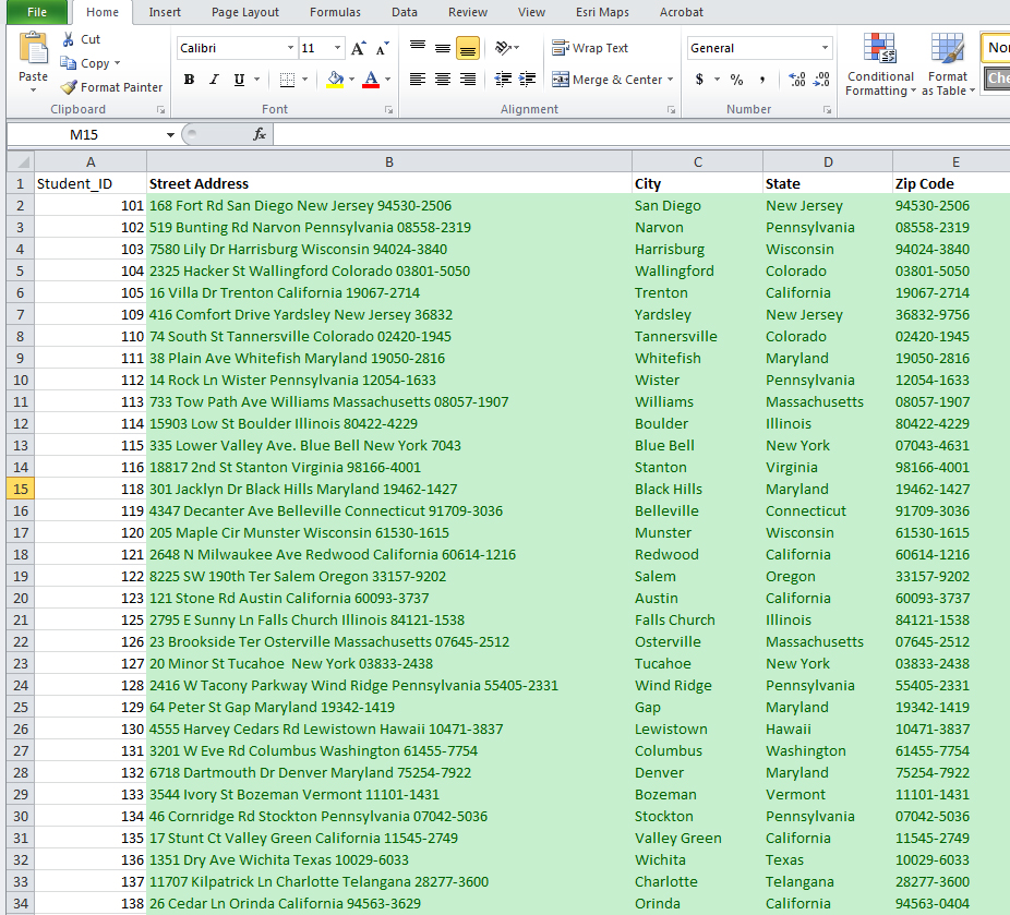
Step 1, Plotting the Points: We start with a spreadsheet that contains individual records that include an associated street address. In this case the address should be divided up into multiple columns (for street address, city, state, zip code). The spreadsheet containing these records must be saved in CSV format so it can be uploaded to QGIS and geocoded.
To upload and geocode the file, the MMQGIS plugin must be installed in QGIS. This is done by selecting “plugins” from the menu and installing MMQGIS using the “Managing and Installing Plugins” option. The menu bar will now include an MMQGIS heading which contains a “Geocode” option. After selecting “Geocode CSV with Google” a window will appear asking for the location of the CSV file. Once selected, you will need to define the address field, state field, city field and country field (if applicable) using the drop down menus. You also need to define the directory location where you want the shape output file as well as the list of any “not found” addresses. After clicking on “OK” the addresses will be geocoded, and their locations plotted on the screen. The layer (a .shp file) will show up in the left hand column of the window with the same name as the original CSV file. 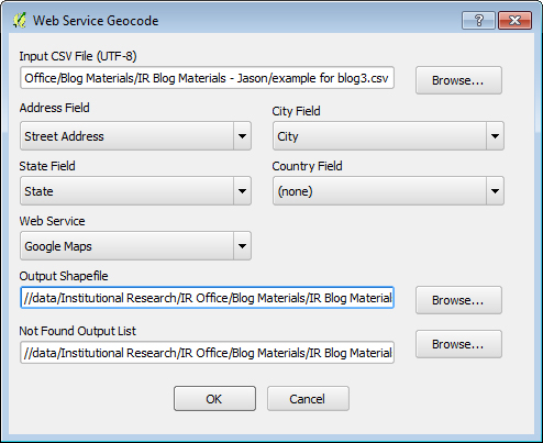
Step 2, Uploading a Geographic Boundary File: Now that the points have been plotted, we can introduce geographic boundaries to the map. The most convenient way to find and download these “shape files” is through the US Census Bureau’s website. There are many options for downloading geographic shape files (called TIGER products by the Census Bureau) including zip code boundaries, municipal boundaries, Congressional District boundaries, etc. In this case, I have chosen to select a Census Tract shape file that includes all of the tracts in the 50 states and Puerto Rico. Here is the link to the specific download:
http://www2.census.gov/geo/tiger/TIGER2010DP1/Tract_2010Census_DP1.zip
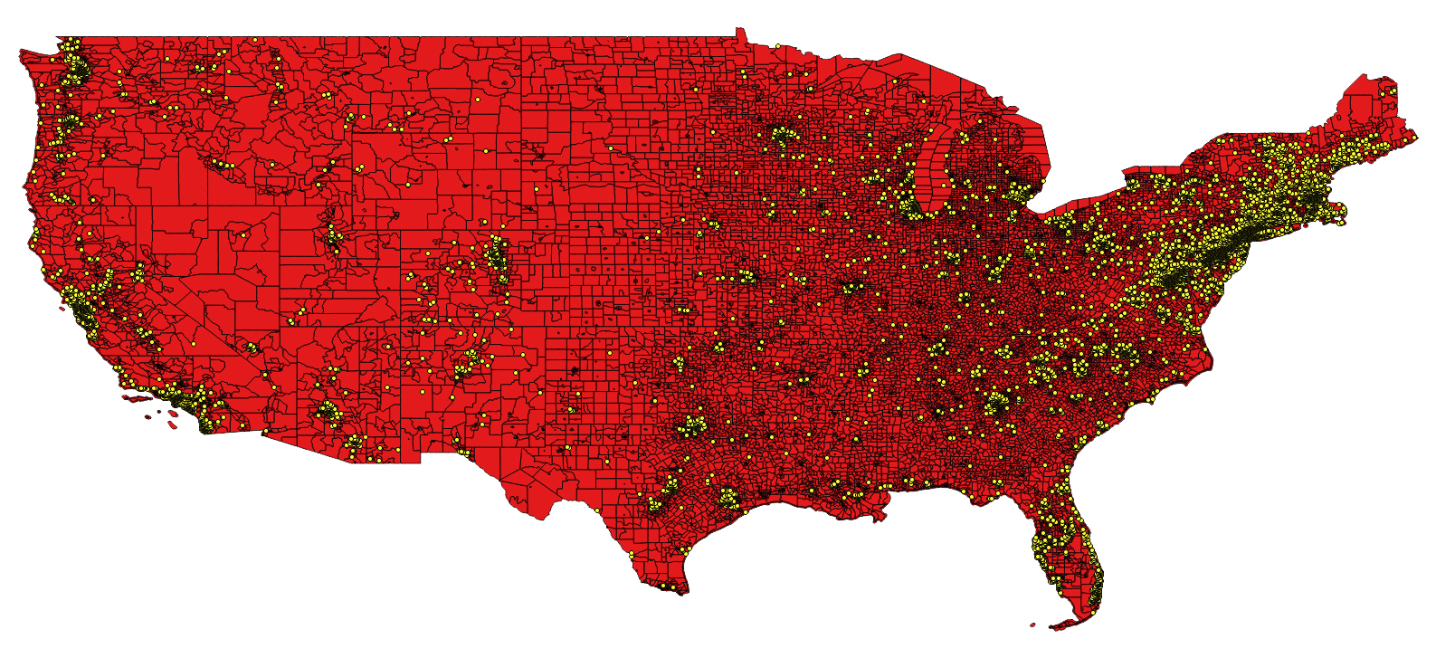
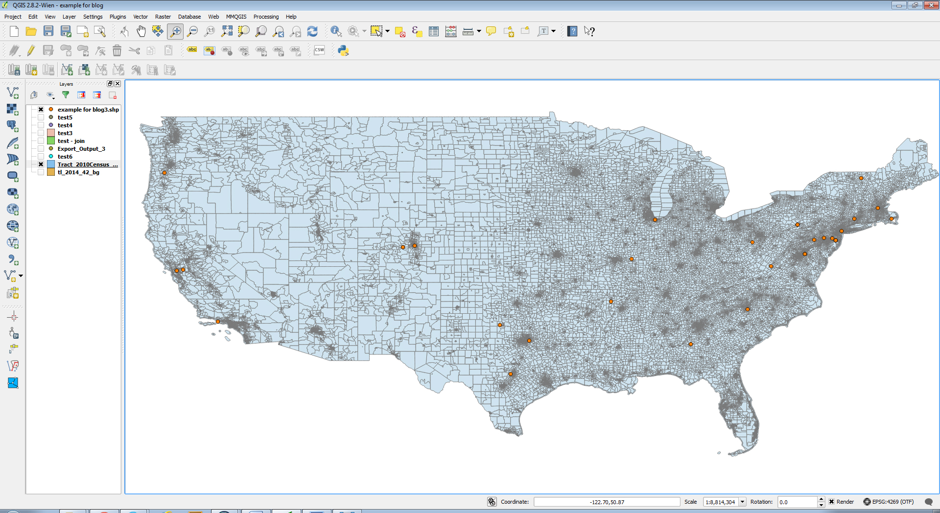
After the zip file has been downloaded to your computer and the files extracted, you can open the shape (selecting the .shp file) from within QGIS. After selecting “Layer” from the menu and “Add Layer” from the sub-menu you are given the option to “Add Vector Layer.” This will allow you to navigate to the .shp document to upload. The map of the United States, including its Census Tract boundaries should appear. You will also notice, if you look closely at the image of the map, the point locations from step one are depicted overtop of the new map.
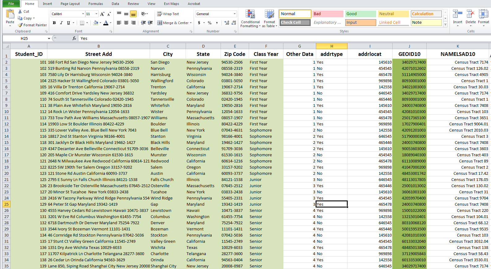
Step 3, the Spatial Join: At this point we have uploaded and depicted both the census tracts and the individual records derived from street addresses. In addition to the depiction of each layer, the file names show up in the left hand column and users can right click and select “Open Attribute Table” to see the underlying data for the depicted layers. This essentially brings up a spreadsheet that contains the data behind the layer. Notice that when we open the attribute table for the census tract file there is a variable called “GEOID10.” This is the geographic identifier for the specific tracts and consists of a two-digit state code, followed by a three-digit county code, followed by a six-digit tract code. This identifier, sometimes called a FIPS code, can be used to connect tract level Census data to descriptions/characteristics of the tract.
A “spatial join” allows us to add the location descriptor (e.g. the GEOID10 FIPS code) to each of the individual point locations by determining which tract it falls inside and then adding the appropriate FIPS to each individual record containing a street address. To carry out the spatial join, select (from the menu) “vector,” then “data management tools,” then “join attributes by location.” There are a few options here, but the most important thing is to select the layer depicting the point locations as the “Target vector layer,” and the Census Tract boundary file as the “Join vector layer.” It will also ask you to provide a name and location on your hard drive for the output .shp file where it will save the combined file. When the spatial join is complete, it will ask if you want to add the new layer to the current map. If you say “yes” and then open the attribute table, you will see your original list of individuals with street addresses and additional columns added including the FIPS code identification of the associated Census Tract.
Step 4, Downloading Joined Data and Merging with Census data: In order to download the spreadsheet in CSV format, you can use the MMQGIS menu, under which there is an import/export option. If you select “Attributes Export to CSV file” you can choose the layer you wish to export.
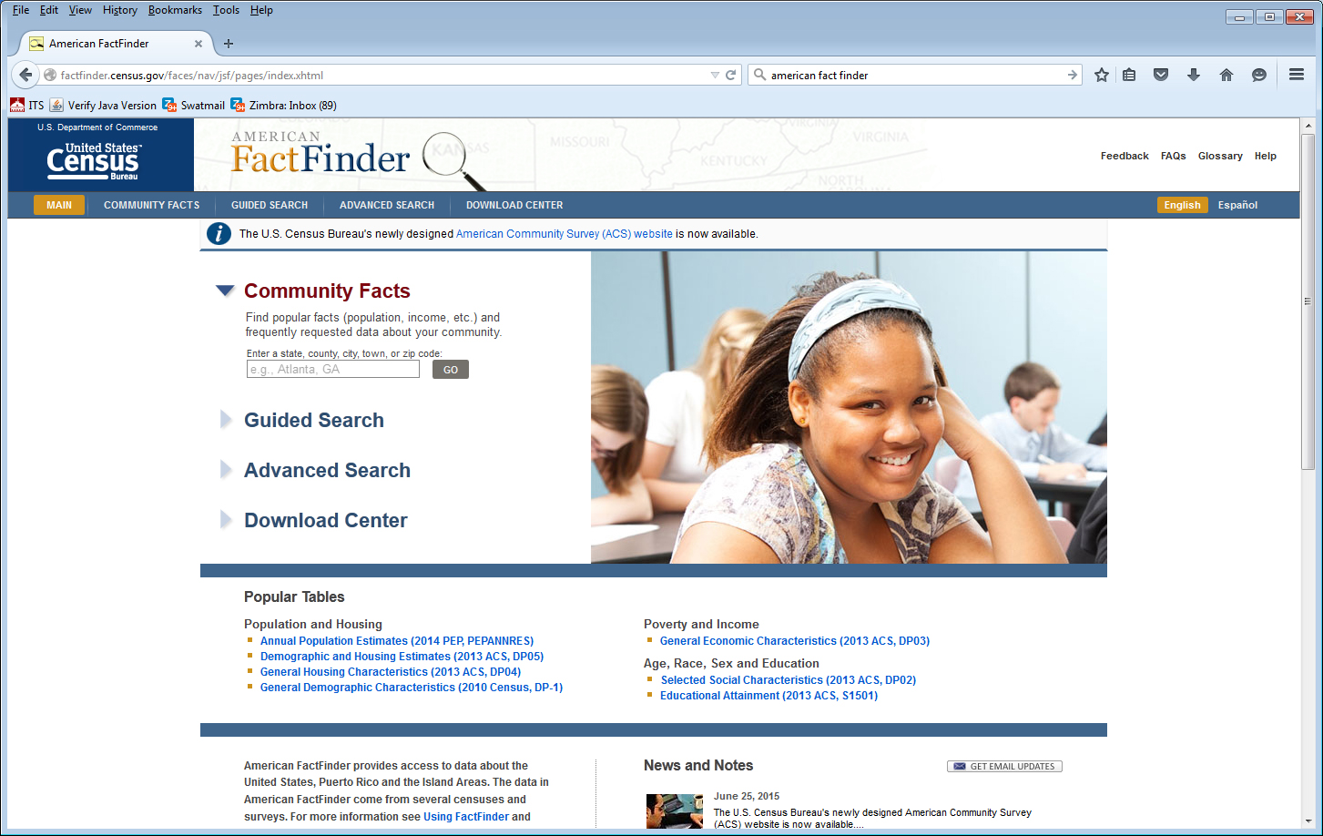
Now that you have a CSV file with a geographic identifier added to the original records you can merge any tract level Census Data (or any tract level data that contains identifying FIPS codes) that has been collected and made available at the tract level. To access tract level data from the U.S. Census, you can go to the Census’ American Fact Finder site and navigate your data download either through the “guided search” or the “advanced search.”
http://factfinder.census.gov/faces/nav/jsf/pages/index.xhtml
When you have chosen tract level data to be downloaded, you can then merge this data with the individual records using SPSS, SAS, Microsoft Access or whatever is your software of choice for merging data based on a unique identifier.