Part Two: From Geographic Location to Neighborhood Profile
In Part One of this two part blog post I explained how to start with a list of street addresses and, using Google’s Fusion Tables function, map those locations onto an interactive Google Map. This tool alone can be very useful and powerful in the context of institutional research and administration. However, where spatial analysis becomes significantly more powerful is when you use these known locations to find out more information about the specific communities and neighborhoods of students and alumni. Through the use of spatial analysis software, these “point” locations can be tied directly to zip codes, census tracts, block groups, Congressional districts, etc. From there, geographic data from the Census Bureau’s American Community Survey or other sources can be used to understand a great deal about where the community and neighborhood profile of students and alumni. It’s only a proxy for the individual and we always need to be aware of the Ecological fallacy, but you can gain immense and detailed understanding of a group just by learning about their spatial location.
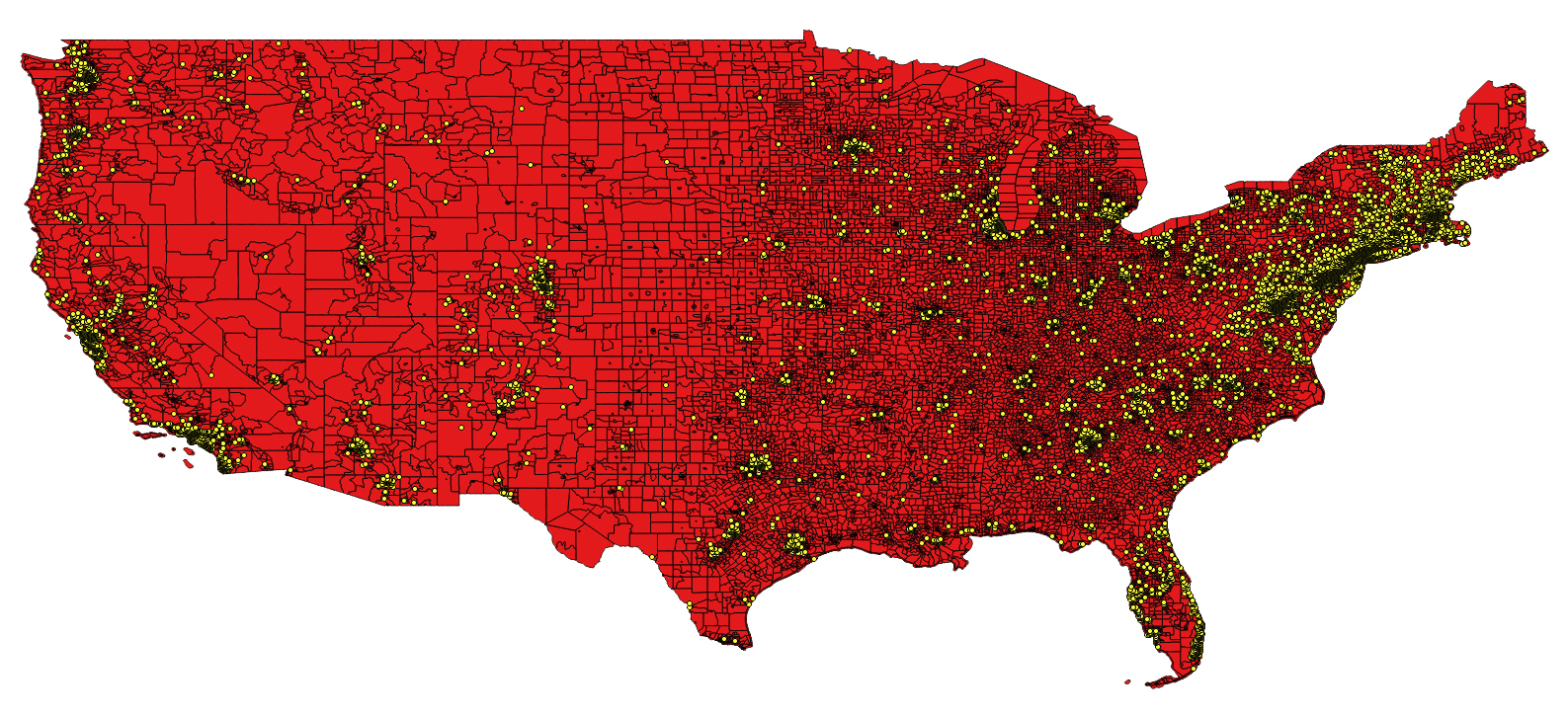
The following is a guide for taking individual records (including street addresses), overlaying geographic boundaries (such as tracts, zip codes, etc.), joining (or combining) the individual records with their respective geographic descriptors (e.g. Student A lives in zip code 12345), and finally, joining/combining geography-based data from the US Census’ American Community Survey to those individual records (e.g. Student A lives in zip code 12345, which has a population of 3,500, a median household income of 65,000 dollars per year, and so on).
